Benchmark of Global Optimization Approaches for Nano-optical Shape Optimization and Parameter Reconstruction
This blog post is based on the publication P.-I. Schneider, et al. Benchmarking five global optimization approaches for nano-optical shape optimization and parameter reconstruction.ACS Photonics 6, 2726 (2019).
DOI: 10.1021/acsphotonics.9b00706
Several global optimization methods for three typical nano-optical optimization problems are benchmarked: particle swarm optimization, differential evolution, and Bayesian optimization as well as multistart versions of downhill simplex optimization and the limited-memory Broyden–Fletcher–Goldfarb–Shanno (L-BFGS) algorithm. In the shown examples, Bayesian optimization, mainly known from machine learning applications, obtains significantly better results in a fraction of the run times of the other optimization methods.
This document is the unedited Author's version of a Submitted Work that was subsequently accepted for publication in ACS Photonics, copyright © American Chemical Society after peer review. To access the final edited and published work see https://doi.org/10.1021/acsphotonics.9b00706.Contents
1 Introduction
Numerical optimization is a fundamental task for many scientific and industrial applications. It is also an important tool in the field of nano-optics. Modern nano-processing technologies such as laser writing [1] or 3D in-situ electron-beam lithography [2, 3] enable the fabrication of micro- and nano-optical structures with an increasing degree of accuracy and flexibility. From an experimental and technological perspective it is often not clear, which geometries and geometrical parameters lead to optimal results in terms of a desired functionality. Numerical simulation and scans of selected parameters can give important insights [4, 5, 6, 7]. However, the full exploitation of the fabrication flexibility requires the simultaneous numerical optimization of all degrees of freedom. This process can be very time consuming and prompts for large computing resources (e. g. multi-core computers or computer clusters), fast simulation methods, and efficient numerical optimization methods that require as few as possible simulation runs of the actual forward problem [8].
Another important application for numerical optimization is the parameter reconstruction based on measured data [9]. For example, optical scatterometry is the state-of-the-art optical inspection technique for quality control in lithographic processing [10]. This indirect measurement procedure relies on a parametrization of the specimen’s geometry and a numerical simulation of the measurement process. Based on multiple numerical simulations, one tries to identify the parameters that match best the measured data. Especially, for in-line quality control it is crucial to find the parameters with as few simulation runs as possible.
In each optimization scenario the first step is to define an objective function that maps the system’s parameters to an objective value that is to be minimized. In nano-optics the computation of the objective function generally requires to solve Maxwell’s equations. This can be achieved by different numerical methods depending on the geometry, such as the Finite-Element Method (FEM), rigorous coupled wave analysis (RCWA), and Finite-Difference Time-Domain (FDTD) method. In this work we use the software package JCMsuite [11], which employs the FEM approach in the frequency domain [12]. Typical computation times range from a few seconds for simple and highly symmetric systems to hours or even days for complex three-dimensional geometries with a spatial extent larger than many wavelengths. Nano-optical systems are often characterized by interference and resonance phenomena. Typically, by varying the dimensions of the system or the wavelength of the light, multiple resonances can be observed. As a consequence, the objective function features in general many separated minima, which makes it difficult to find the global minimum. This is, for example, in contrast to the optimization problem of training artificial neural networks, where local minima seem not to be an obstacle in finding optimal network weights [13].
Optimization problems can be roughly divided into low-dimensional problems (1 to 3 parameters), medium-dimensional problems (4 to \(\sim \) 15 parameters) and high-dimensional problems (\(\sim \) 15 parameters to some hundred parameters or more). While low-dimensional problems often allow for scanning the full parameter space, this is already impossible for medium-dimensional problems. E.g., a scan of a 10-dimensional parameter space with a resolution of 100 different values for each parameter requires \(100^{10}=10^{20}\) evaluations of the objective function, rendering a regular parameter scan infeasible. This problem, known as curse of dimensionality, is tackled by global optimization approaches, which try to sample the parameter space in an effective way by avoiding regions with large function values. For high-dimensional problems, as they appear for example in the context of topology optimization, a global optimization is often impossible due to the exponentially growing number of possible parameter values to test. In this case, one often resorts to a local optimization method that explores the parameter space starting from a given initial parameter vector [14, 15, 16] or one considers a discretization of the parameter space and applies evolutionary optimization techniques [17, 18]. Alternatively, one can recast the optimization problem by searching for an optimal material distribution using algorithms such as ADMM or successive convex approximations, while treating the Maxwell equations as a constraint [19, 20, 21].
In this work, we focus on medium-dimensional optimization problems that allow for a global optimization of parametrized geometries based on the solution of Maxwell’s equations, but do not allow for a complete scan of the parameter space. We consider two shape-optimization problems, i.e. the optimization of an integrated single-photon source and the optimization of a dielectric metasurface. Further, we consider the problem of a geometrical parameter reconstruction based on X-ray diffraction measurements.
We benchmark optimization algorithms that are regularly applied in nano optics and that can be broadly assigned to three categories: local optimization, global stochastic optimization, and global model-based optimization.
• Starting from a given initial parameter vector, local optimization methods try to find better positions in the parameter space by exploring the neighborhood of the current position. They converge efficiently into a local minimum, which is not necessarily the global minimum. Gradient-based methods use first derivatives (gradients) or second derivatives (Hessians) in order to find a minimum in a smaller number of iterations. An example for a gradient-free method is the downhill simplex algorithm [22] and an example for a gradient-based method is the low-memory Broyden-Fletcher-Goldfarb-Shanno (L-BFGS-B) algorithm [23]. The gradient of the solution to Maxwell’s equations can be obtained by the adjoint method [24, 16] or by automatic differentiation [25]. Local optimization methods have been used, e.g., to optimize a Y-junction splitter [24] or a photonic nano-antenna [26], and to reconstruct geometrical parameters of a line grating from scatterometry data [25].
• Stochastic optimization algorithms are based on random variables. Important representatives are particle swarm optimization [27] and differential evolution [28]. These algorithms usually scale well for an increasing number of dimensions. However, they tend to require many function evaluations in order to converge to the global minimum. Particle-swarm optimization has been employed for optimizing diffraction grating filters [29], photonic-crystal waveguides [30], or the duality symmetry of core-shell particles [31]. Differential evolution strategies have been investigated in the context of light focusing photonic crystals [32] and for parameter extraction of optical materials [33].
• Model-based optimization methods construct a model of the objective function in order to find promising sampling parameters. One important representative is Bayesian optimization, which constructs a statistical model of the objective function [34]. Bayesian optimization is regularly used in machine learning applications [34, 35, 36]. In the field of nano-optics it has been employed to optimize ring resonator-based optical filters [37], chiral scatterers [38], and mantle cloaks [39]. The method derives promising parameter samples by means of Bayesian inference based on all previous function evaluations. This is in contrast to the other approaches, which only use few historic data points to determine new samples. While this statistical inference can drastically reduce the number of iterations, it requires a significant computational overhead on its own, which can slow down the optimization. We introduce an approach that aims to eliminate this slow-down for typical nano-optical computation scenarios.
Another machine-learning technique that has been recently applied for nano-optical optimization is deep learning [40]. Trained with thousands of simulation results deep neural networks can serve as accurate models for mapping a geometry to an optical response and vice versa almost instantaneously. However, for this benchmark we only consider methods that do not require a training phase prior to the actual optimization.
2 Examined optimization methods
In the field of optical simulations one has often access to computing clusters or powerful multi-core computers. It is therefore important that optimization methods exploit the possibility of computing the objective function for several input values in parallel. Moreover, it should be possible to distribute the computation of the objective function to several machines or threads. To this end, we have integrated the considered optimization methods in a server-client framework following the design strategy of Google Vizier [35]. Furthermore, we adapted the optimization methods to support inequality constraints of the parameter space that arise from geometrical or practical (e.g. fabrication) requirements.
In the following, we shortly describe the optimization approaches. Further details on the numerical framework, the implementation of the algorithms supporting a constrained optimization as well as a visualization of the different optimization strategies are contained in the Supporting information.
2.1 Local optimization methods
In local optimization methods, the next sampling point depends on the function value of the previous sample. A parallelization of local optimization methods is achieved by starting several independent local optimizations from different pseudo-random points in the parameter space \(\mathcal {X} \subset \mathbb {R}^D\). After a local optimization has converged, it is restarted from a different point such that eventually the global minimum would be found.
For optimization problems that do not exploit derivative information, we consider the downhill simplex algorithm [22]. Otherwise, we consider the gradient-based L-BFGS-B algorithm [23]. Both methods are implemented based on the python package scipy.optimize [41].
2.2 Stochastic global optimization
As stochastic global optimization methods, we consider particle swarm optimization and differential evolution.
Particle swarm optimization works by randomly moving the position of each particle in the search-space guided by the particle’s best known position as well as the swarm’s best known position. The method is implemented based on the Python package pyswarm [42], which supports a parallel evaluation of the objective function.
Differential evolution is a population-based genetic algorithm that is implemented based on the python package scipy.optimize.differential_evolution [41, 43]. We extend the algorithm by allowing for a parallel evaluation of the fitness function for each offspring.
The performance of the stochastic global optimization algorithms heavily depends on parameters such as the swarm size and the population size (see supporting information for a comparison). Due to the computational complexity of adapting these parameters, the benchmark is performed with the default parameters of the python packages.
2.3 Bayesian optimization
Bayesian optimization is based on a stochastic model of the objective function. We employ a Gaussian process (GP) that is updated with each new evaluation of the objective function through GP regression (a form of Bayesian inference) [44, 34]. The GP allows to identify parameter values with the largest expected improvement \({\rm EI}(\mathbf {x})\). By sampling those points, exploitation and exploration are automatically balanced, i.e. after exploiting a possible improvement within a local minimum, other parts of the parameter space are automatically scanned until a better minimum is found. As proposed by Gonzales et al. [45] the parallelization is realized by penalizing the expected improvement of the parameters close to running calculations.
One important advantage of GP regression is that it does not rely on derivative information on the objective function, but that one can incorporate this information if available [46]. We use an in-house implementation of Bayesian optimization that exploits the possibility to include derivative observations [47]. As will be shown below, this can speed up the optimization significantly.
The search process for the next sampling point is itself an optimization problem that can be computationally demanding and may slow down the optimization. To tackle this problem in the context of parallel computations of the objective function, we use two strategies: (i) The next sampling point is computed in advance, i.e. in parallel to the evaluation of the objective functions. (ii) We use differential evolution to maximize the expected improvement and automatically adapt the effort to the average time interval at which new objective function values are acquired. See the supporting information for a detailed description of the approach.
3 Optimization Problems
For benchmarking the different optimization algorithms, we consider three technologically relevant optimization problems of contemporary interest: the maximization of the coupling efficiency of a single-photon source to an optical fiber, the parameter reconstruction of a lamellar grating from scattering data, and the reflection suppression from a silicon metasurface. These three problems are described in the following individually prior discussing the results from the optimization.
3.1 Improving the coupling efficiency of a single-photon source
a)

b)

c)

Figure 1: a) Visualization of the energy density of the light field of the optimized fiber-coupled single-photon source with a coupling efficiency of 60%. A cut through the geometry is shown in front of the energy-density plot. The single-photon source consists of a QD dipole source embedded into a mesa structure (GaAs, blue), a Bragg reflector [alternating layers of GaAs (blue) and Al0.9 Ga0.1 As (gray)], and an optical fiber with homogeneous fiber core (orange) and fiber cladding (yellow). The Bragg reflector is grown on a substrate made of GaAs and has a GaAs top layer (blue). The six optimized parameters are the mesa height \(h_{\rm mesa} = 1217\,{\rm nm}\), mesa radius \(r_{\rm mesa} = 522\,{\rm nm}\), top-layer thickness \(h_{\rm layer} = 190\,{\rm nm}\), dipole elevation within the mesa \(h_{\rm dip} = 613\,{\rm nm}\), fiber-core radius \(r_{\rm core} = 969\,{\rm nm}\) , and mesa-fiber distance \(s_{\rm mf} = 352\,{\rm nm}\). b): Best seen coupling efficiency for different optimization approaches as a function of the number of simulations averaged over six independent optimization runs. The shading indicates the standard error, i. e. the uncertainty of the average. c): Same as b) but the best seen coupling efficiency is shown as a function of the total computation time. The comparison with a) shows that Bayesian optimization has no significant computational overhead compared to the other optimization approaches.
Single-photon sources are essential building blocks of future photonic and quantum optical devices. We consider a source consisting of a quantum dot (QD) emitting at a vacuum wavelength of \(\lambda =1,300\,\)nm in the telecom O-band. The QD is embedded into a mesa structure made from gallium arsenide (GaAs; refractive index \(n_{\rm GaAs} = 3.4\)). An underlying Bragg reflector made from layers of GaAs and aluminum gallium arsenide (Al0.9 Ga0.1 As; \(n_{\rm AlGaAs}=3.0\)) reflects the light emitted by the QD back into the upper hemisphere. The light is coupled into an optical fiber with large numerical aperture (NA) above the QD consisting of a homogeneous fiber core and a homogeneous fiber cladding (\(n_{\rm core} = 1.5\), \(n_{\rm clad} = 1.45\), \({\rm NA} \equiv \sqrt {n_{\rm core}^2-n_{\rm clad}^2} = 0.38\)). The setup is sketched in Fig. 1 a).
The parameter space \(\mathcal {X}\) is spanned by 6 parameters: the height of the top layer above the Bragg reflector (\(h_{\rm layer}\)), the radius of the fiber core (\(r_{\rm core}\)), the radius and height of the mesa (\(r_{\rm mesa}\), \(h_{\rm mesa}\)), the elevation of the dipole within the mesa (\(h_{\rm dip}\)), and the distance between mesa and fiber (\(s_{\rm mf}\)). The objective of the optimization is to maximize the coupling efficiency of the emitted light into the fundamental modes of the fiber. The numerical method to determine the coupling efficiency was described by Schneider et al. [48].
3.2 Parameter reconstruction of a lamellar grating
Grazing incidence small angle X-ray scattering (GISAXS) is a destruction-free scatterometry method. With incidence angles close to the critical angle of total external reflection, GISAXS is a technique with high surface sensitivity. We consider the parameter reconstruction of a periodic, lamellar silicon grating manufactured using electron beam lithography [49]. The grating geometry is modeled by 5 parameters: the critical dimension \(\rm CD\) (line width), the line height \(h_{\rm line}\), the side-wall angle \(\phi _{\rm swa}\), the top corner radius \(r_{\rm top}\), and the depth of the grooves \(d_{\rm groove}\) [see Fig. 2 a)]. A monochromatic X-ray beam idealized as a plane wave with the wave vector \(\mathbf {k}_{\rm in}\) impinges on the sample surface at a grazing incidence angle. The elastically scattered wave with the wave vector \(\mathbf {k}_{\rm f}\) propagates to a 2D area detector that records a scattering intensity pattern \(I_{\rm det}(\mathbf {q})\) as a function of the scattering vector \(\mathbf {q} = \mathbf {k}_{\rm f} - \mathbf {k}_{\rm in}\) [see Fig. 2 b)]. Based on a FEM model of the experiment, one can determine a scattering intensity \(I_{\rm FEM}(\mathbf {p},E,N)\) for each parameter set \(\mathbf {p}\in \mathcal {X}\), photon energy \(E\), and diffraction order \(N\) [49].
The natural line edge and line width roughness of the grating is taken into account with an analytic approach based on Debye-Waller damping \(\exp (-[\sigma _{\rm r} \mathbf {q}_y(N)]^2)\) with the damping factor \(\sigma _{\rm r}\) and the \(y\)-component \(\mathbf {q}_y(N)\) of the scattering vector for diffraction order \(N\). Furthermore, the model intensities are scaled by an energy-dependent factor \(s(E)\) in order to account for the unknown effective illumination area of the sample. This leads to the model \(I_{\rm model}(\mathbf {p},E,N) = I_{\rm FEM}(\mathbf {p},E,N)\, s(E)\, \exp (-[\sigma _{\rm r} \mathbf {q}_y(N)]^2)\) for the measured intensities in each diffraction order \(N\).
The data acquisition is performed for three different photon energies, \(E_1 = 5.5\,{\rm kEV}\), \(E_2 = 5.55\,{\rm kEV}\), and \(E_3 = 5.6\,{\rm kEV}\). For each energy, the standard deviation \(\sigma (E_i)\) of the measured intensities was determined, as described by Soltwisch et al. [49]. The aim of the optimization is to minimize the mean squared numerical error of all diffraction orders and energies
\begin{equation} \label {eq:chi_squared} \chi ^2 = \sum _{i=1}^3 \sum _{N=1}^M \frac {\left ( I_{\rm model}(\mathbf {p},E_i,N) - I_{\rm exp}(E_i,N) \right )^2}{\sigma ^2(E_i)} \end{equation}
with respect to the geometrical parameters \(\rm CD\), \(h_{\rm line}\), \(\phi _{\rm swa}\), \(r_{\rm top}\), \(d_{\rm groove}\), the roughness \(\sigma _{\rm r}\), and the three scaling factors \(s_i = s(E_i)\) for \(i=1,2,3\).
We note, that it is straightforward to determine the derivatives of \(\chi ^2\) with respect to the parameters \(\sigma _{\rm r}\), \(s_1\), \(s_2\), and \(s_3\) that do not enter into the numerical FEM simulation of the measurement process. In the next section we will make use of these derivative information in order to assess to which extend partial information on parameter derivatives can speed up the Bayesian optimization process.
a)

b)

c)

d)

Figure 2: a) Geometry of the lamellar grating. The aim of the GISAXS measurement is to reconstruct the critical dimension \(\rm CD\), the line height \(h_{\rm line}\), the side-wall angle \(\phi _{\rm swa}\), the top corner radius \(r_{\rm top}\), and the depth of the grooves \(d_{\rm groove}\). b) GISAXS scattering pattern of the grating obtained at a photon energy of 6.5 keV shown as a function of the scattering vector components \(\mathbf {q}_y\) and \(\mathbf {q}_z\). The intensity is shown with a logarithmic false color scale. c): Error \(\chi ^2\) [see Eq. (1)] for different optimization approaches as a function of the median number of simulations needed to reach a value below \(\chi ^2\) for six independent optimization runs. The blue and green lines show the results of Bayesian optimization including derivatives and using no derivative (n.d.) information, respectively. d): Same as c) but \(\chi ^2\) is shown as a function of the median total computation time.
3.3 Reflection suppression by a metasurface
Broadband anti-reflection is a desirable property, e.g., for high-efficiency solar cells as well as for CCD or CMOS sensors. We consider a nano-structured silicon metasurface for suppressing the reflectivity in a broad range of frequencies [50]. The metasurface consists of a square array of silicon bumps on top of a silicon substrate [see Fig. 3 a)] and is parametrized by six length scales: the periodicity of the array (\(p\)), the heights of the lower and upper part of the bumps (\(h_{\rm lower}\), \(h_{\rm upper}\)), and the bottom, middle, and top width of the bumps (\(w_{\rm bottom}\), \(w_{\rm middle}\), \(w_{\rm top}\)). The reflectivity of incident plane waves perpendicular to the surface is averaged over four wavelengths, \(500\,{\rm nm}\), \(600\,{\rm nm}\), \(700\,{\rm nm}\), and \(800\,{\rm nm}\). In order to facilitate the fabrication of the structure we constrain the parameter space of the optimization such that \(w_{\rm bottom} \leq p - 10\,{\rm nm}\), \(w_{\rm bottom} \leq w_{\rm middle} \leq w_{\rm top}\) and \(h_{\rm lower} + h_{\rm upper} \leq 2 w_{\rm bottom}\).
a)

b)

c)

Figure 3: a): The metasurface consists of a square array of silicon bumps on a silicon substrate. The reflectivity of the structure is minimized with respect to the periodicity of the array (\(p\)), the heights of the lower and upper part of the bumps (\(h_{\rm lower}\) and \(h_{\rm upper}\)), and the bottom, middle, and top width of the bumps (\(w_{\rm bottom}\), \(w_{\rm middle}\), and \(w_{\rm top}\)). b): Lowest reflectivity for different optimization approaches as a function of the number of simulations averaged over six independent optimization runs. The shading indicates the standard error. c): Same as b) but the lowest reflectivity is shown as a function of the total computation time. Bayesian optimization using no derivative information ["Bayesian optimization (n.d.)"] takes roughly twice as long to obtain a reflectivity below 1%.
Using automatic differentiation, the FEM software JCMsuite [11] allows to determine partial derivatives of the computed fields with respect to geometrical parameters with small computational overhead. Based on this information, we compute for this example the partial derivatives of the reflectivity with respect to the six design parameters.
4 Numerical experiments
The optimization runs for the three optimization problems introduced in the previous section have been each performed for a fixed number of iterations (single-photon source optimization and parameter reconstruction 2,500 iterations, anti-reflective metasurface optimization 500 iterations). In order to evaluate the average performance of the different optimization methods, each run has been repeated 6 times with different initial conditions. All methods were run with typical numerical settings (see supporting information). A targeted adaptation of the settings to a specific optimization problem is generally computationally much more demanding than the optimization problem itself [51]. In practice, the problem-adapted performance is therefore usually less relevant than the performance with default parameters.
In addition to the optimization methods introduced in the first section, results for a random sampling of the objective functions are also considered. If an optimization method is not significantly better than the non-informative random sampling, it suffers from the specific properties of the objective function, e.g. irregularities or the existence of too many local minima.
The optimization of the single-photon source and the parameter reconstruction were performed on a machine with a 6-core Intel Xeon CPUs running at 3.2 GHz with 11 GB of RAM. The optimization methods were configured to perform at most 4 parallel computations of the objective function. The optimization of the metasurface is numerically much more demanding as a three-dimensional geometry is considered and a wavelength scan has to be performed. Therefore, the optimizations were run on a more powerful machine with 4 Intel Xeon CPUs with 10 cores at 2.4 GHz with 1 TB of RAM. Up to 6 parallel computations of the objective function were performed. On both machines Bayesian optimization used four parallel threads for computing the sampling points.
4.1 Optimized single-photon source
Figure 1 b) and c) compares the performance of Bayesian optimization, particle swarm optimization, differential evolution, the downhill simplex method, and random sampling for the example of the maximization of the coupling efficiency of the emitted light into the optical fiber. Bayesian optimization clearly outperforms all other methods. After about 1,200 iterations and a computation time of 6 hours it reaches an average coupling efficiency of 55% while the other optimization methods reach only average efficiencies below 52% after 2,500 iteration and a computation time of 12 hours. A comparison of Figs. 1 b) and c) shows that Bayesian optimization has no significant computational overhead compared to the other optimization approaches.
The computed optimal configuration with mesa height \(h_{\rm mesa} = 1217\,{\rm nm}\), mesa radius \(r_{\rm mesa} = 522\,{\rm nm}\), top-layer thickness \(h_{\rm layer} = 190\,{\rm nm}\), dipole elevation \(h_{\rm dip} = 613\,{\rm nm}\), fiber-core radius \(r_{\rm core} = 979\,{\rm nm}\), and mesa-fiber distance \(s_{\rm mf} = 352\,{\rm nm}\) is shown in Fig. 1 a). The setup achieves a remarkably large coupling efficiency of 60% to the optical fiber. In a previous work, we tried to improve the coupling efficiency of the same system by performing numerical scans of all parameters of the geometry apart from the top-layer thickness \(h_{\rm layer}\), which was fixed to 195 nm. A full parameter scan of all five parameters with only 10 values per parameter would have required 100,000 simulations. Therefore, we restricted in the prior work the scan to a small fraction of the physically realizable parameter space. For example, dipole elevations only between 0 and 50 nm in steps of 10 nm were considered, while the current optimization considers values between 0 and 1000 nm. Due to this restriction, a maximal coupling efficiency of only 23% had been obtained in the past [48]. This demonstrates that an optimization within a large space of realizable system parameters is important to assess the technological potential of a nano-optical system.
4.2 Parameter reconstruction of a lamellar grating
For practical applications of shape optimization it is of interest to determine a reasonably good structure in a limited time budget (e.g. in one day). In contrast, in the context of a parameter reconstruction it is important to find parameter values close to the global optimum with a small error level \(\chi ^2\) as fast as possible. Correspondingly, Fig. 2 c) and d) show the median number of simulations and the median time span needed to reach a specific error level \(\chi ^2\). The optimal parameters correspond to the values obtained by Soltwisch et al. [49].
In this case, Bayesian optimization shows an impressive lead in comparison with the other optimization methods. Using the derivative information with respect to the parameters \(\sigma _{\rm r},s_1,s_2,s_3\), Bayesian optimization reaches an error level of \(10^3\) after a median number of about 200 simulations and a median time of one hour (blue line), while the non-Bayesian methods do not manage to reach the same error level even after 2,500 iterations or eight hours computation time.
4.3 Optimized anti-reflective metasurface
For the example of the reflection suppression using a metasurface, all first order partial derivatives with respect to the six geometrical parameters were determined by automatic differentiation. This enables to apply also the gradient-based L-BFGS-B method. The benchmark results are presented in Figs. 3 b) and c). Again Bayesian optimization, even without using derivative information ["Bayesian optimization (n.d.)"], optimizes the structure significantly faster. It reaches average reflectivities below 0.5% while Differential evolution obtaines 0.7% and the other optimization methods between 1% and 2%. The use of derivatives for Bayesian optimization offers again a significant advantage. It is remarkable that this is not the case for L-BFGS-B optimization. After a relatively fast initial optimization to 5% reflectivity, L-BFGS-B performs comparable to the other non-derivative methods, including random sampling. We attribute this to a complex shape of the objective function with many similarly low local minima.
The best geometry with the parameter values \(h_{\rm lower} = 225\) nm, \(h_{\rm upper} = 244\) nm, \(w_{\rm bottom} = 244\) nm, \(w_{\rm middle} = 204\) nm, \(w_{\rm top} = 57\) nm, and \(p = 254\) nm has an objective value of 0.27% reflectivity. In Fig. 4, the optimal geometry is shown together with a full wavelength scan of its reflectivity in the range of 400 nm to 900 nm. As expected, the reflectivity outside the optimization range of 500 nm to 800 nm increases significantly. Still, the average reflectivity in the range of 400 nm to 900 nm is only 0.71%.
In a previous numerical study on the same silicon metasurfaces a significantly higher minimal averaged reflectivity of 4% was reached in the range of 400 nm to 900 nm by means of parameter scans within a three-dimensional parameter space (periodicity of square array, width and height of silicon bumps) [50]. This again demonstrates, that an optimization within a larger parameter space can significantly improve the performance of nano-optical structures with respect to parameter scans in a small subspace.
a)
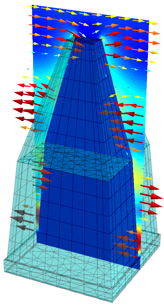
b)

Figure 4: a): Optimal geometry of a single bump of the square lattice with \(h_{\rm lower} = 225\) nm, \(h_{\rm upper} = 244\) nm, \(w_{\rm bottom} = 244\) nm, \(w_{\rm middle} = 204\) nm, \(w_{\rm top} = 57\) nm, and \(p = 254\) nm. Note that the periodicity \(p\) is only 10 nm larger than the bottom width \(w_{\rm bottom}\) of the bumps. Furthermore, the electric field is visualized by an intensity profile and electric field vectors evincing large field intensity in the gaps between the bumps. b): Wavelength scan of the reflectivity for the optimized structure. The metasurface has an average reflectivity 0.19% in the wavelength range of 500 nm to 800 nm and 0.71% in the range of 400 nm to 900 nm.
5 Conclusion
We compared five state-of-the-art optimization methods and applied them to three characteristic nano-optical optimization problems: the maximization of the coupling efficiency of a single-photon source, the reconstruction of geometrical parameters based on scatterometry data, and the suppression of the reflectivity of a silicon metasurface. The optimization methods were extended to meet typical requirements of computational nano-optics, e.g. several objective function values can be computed in parallel. All methods were run with typical numerical settings, i.e. without a manual targeted adaptation to the optimization problems.
The numerical experiments showed that Bayesian optimization reaches good objective function values in only a fraction of the run times of the other considered methods, downhill simplex optimization, L-BFGS-B, particle swarm optimization, and differential evolution. The use of derivative information with respect to some or all parameters can further reduce the run times of Bayesian optimization. The method can require a significant computational overhead for finding parameter samples with a large expected improvement. However, a corresponding prolongation of the total optimization time could be prevented by computing the next sample in advance and by adapting the effort for finding the sample to the effort of computing the objective function. While this means that the quality of the samples decreases if they are requested at a high frequency, Bayesian optimization offers a significant performance gain over other methods even for frequencies of more than one sample every 20 seconds (single-photon source optimization and parameter reconstruction). Hence, the method is likely to be advantageous for many 2D and almost all 3D simulation problems. We note, however, there can be situations when the considered Bayesian optimization is inefficient. This is, e.g., the case if the underlying Gaussian process regression is inaccurate due to irregularities such as discontinuities or sharp resonance peaks of the objective function [52]. Another challenge for Bayesian optimization are high-dimensional optimization problems since the underlying problem of maximizing the expected improvement becomes increasingly hard. The supporting information contains a discussion on Gaussian process regression and its limitations as well as a benchmark study of a high-dimensional optimization problem.
Finally, we note that the properties of the optimized single-photon source and the anti-reflective metasurface are considerably better than those obtained previously from parameter scans. The results suggest that, whenever possible, one should perform global optimizations within the physically feasible parameter space in order to assess the technological potential of a nano-optical structure.
6 Funding Information
This project has received funding from the European Unions Horizon 2020 research and innovation programme under the Marie Sklodowska-Curie grant agreement No 675745 (MSCA-ITN-EID NOLOSS). Further, we acknowledge financial support from the EMPIR programme co-financed by the Participating States and from the European Union’s Horizon 2020 research and innovation programme under grant agreement number 17FUN01 (BeCOMe). We also acknowledge support by KIT through the Virtual Materials Design (VIRT-MAT) project by the Helmholtz Association via the Helmholtz program Science and Technology of Nanosystems (STN).
References
[1] Fischer, J. and Wegener, M., “Three-dimensional optical laser lithography beyond the diffraction limit,” Laser Photonics Rev. 7(1), 22–44 (2011).
[2] Yoon, G., Kim, I., So, S., Mun, J., Kim, M., and Rho, J., “Fabrication of three-dimensional suspended, interlayered and hierarchical nanostructures by accuracy-improved electron beam lithography overlay,” Scientific reports 7(1), 6668 (2017).
[3] Kaganskiy, A., Fischbach, S., Strittmatter, A., Rodt, S., Heindel, T., and Reitzenstein, S., “Enhancing the photon-extraction efficiency of site-controlled quantum dots by deterministically fabricated microlenses,” Opt. Communications 413, 162 – 166 (2018).
[4] Gschrey, M., Thoma, A., Schnauber, P., Seifried, M., Schmidt, R., Wohlfeil, B., Krüger, L., Schulze, J.-H., Heindel, T., Burger, S., Schmidt, F., Strittmatter, A., Rodt, S., and Reitzenstein, S., “Highly indistinguishable photons from deterministic quantum-dot microlenses utilizing three-dimensional in situ electron-beam lithography,” Nat. Communications 6, 7662 (2015).
[5] Chen, Y., Nielsen, T. R., Gregersen, N., Lodahl, P., and Mørk, J., “Finite-element modeling of spontaneous emission of a quantum emitter at nanoscale proximity to plasmonic waveguides,” Phys. Rev. B 81, 125431 (Mar 2010).
[6] Bulgarini, G., Reimer, M. E., Bouwes Bavinck, M., Jöns, K. D., Dalacu, D., Poole, P. J., Bakkers, E. P. A. M., and Zwiller, V., “Nanowire waveguides launching single photons in a gaussian mode for ideal fiber coupling,” Nano Letters 14(7), 4102–4106 (2014).
[7] Yang, J., Hugonin, J.-P., and Lalanne, P., “Near-to-far field transformations for radiative and guided waves,” ACS Photonics 3(3), 395–402 (2016).
[8] Bogaerts, W. and Chrostowski, L., “Silicon photonics circuit design: Methods, tools and challenges,” Laser Photonics Rev. 12(4), 1700237 (2017).
[9] Pang, L., Peng, D., Hu, P., Chen, D., He, L., Li, Y., Satake, M., and Tolani, V., “Computational metrology and inspection (CMI) in mask inspection, metrology, review, and repair,” Adv. Opt. Techn. 1(4), 299–321 (2012).
[10] Bodermann, B., Ehret, G., Endres, J., and Wurm, M., “Optical dimensional metrology at Physikalisch-Technische Bundesanstalt (PTB) on deep sub-wavelength nanostructured surfaces,” Surf. Topogr. 4(2), 024014 (2016).
[11] “JCMsuite - the simulation suite for nanooptics.” https://jcmwave.com (2019).
[12] Monk, P., [Finite Element Methods for Maxwell’s Equations], Clarendon Press (2003).
[13] Goodfellow, I. J., Vinyals, O., and Saxe, A. M., “Qualitatively characterizing neural network optimization problems,” arXiv preprint arXiv:1412.6544 (2014).
[14] Piggott, A. Y., Petykiewicz, J., Su, L., and Vučković, J., “Fabrication-constrained nanophotonic inverse design,” Sci. Rep. 7(1), 1786 (2017).
[15] Christiansen, R., Vester-Petersen, J., Madsen, S., and Sigmund, O., “A non-linear material interpolation for design of metallic nano-particles using topology optimization,” Computer Methods in Applied Mechanics and Engineering 343, 23–39 (2018).
[16] Sell, D., Yang, J., Doshay, S., Yang, R., and Fan, J. A., “Large-angle, multifunctional metagratings based on freeform multimode geometries,” Nano letters 17(6), 3752–3757 (2017).
[17] Hu, J., Ren, X., Reed, A. N., Reese, T., Rhee, D., Howe, B., Lauhon, L. J., Urbas, A. M., and Odom, T. W., “Evolutionary design and prototyping of single crystalline titanium nitride lattice optics,” ACS Photonics 4(3), 606–612 (2017).
[18] Wiecha, P. R., Arbouet, A., Girard, C., Lecestre, A., Larrieu, G., and Paillard, V., “Evolutionary multi-objective optimization of colour pixels based on dielectric nanoantennas,” Nature nanotechnology 12(2), 163 (2017).
[19] Lu, J., Boyd, S., and Vučković, J., “Inverse design of a three-dimensional nanophotonic resonator,” Opt. Express 19, 10563–10570 (May 2011).
[20] Lu, J. and Vučković, J., “Nanophotonic computational design,” Opt. Express 21, 13351–13367 (Jun 2013).
[21] Piggott, A. Y., Lu, J., Lagoudakis, K. G., Petykiewicz, J., Babinec, T. M., and Vučković, J., “Inverse design and demonstration of a compact and broadband on-chip wavelength demultiplexer,” Nature Photonics 9(6), 374–377 (2015).
[22] Nelder, J. A. and Mead, R., “A simplex method for function minimization,” Comput. J. 7(4), 308–313 (1965).
[23] Byrd, R. H., Lu, P., Nocedal, J., and Zhu, C., “A limited memory algorithm for bound constrained optimization,” SIAM J. Sci. Comput. 16(5), 1190–1208 (1995).
[24] Lalau-Keraly, C. M., Bhargava, S., Miller, O. D., and Yablonovitch, E., “Adjoint shape optimization applied to electromagnetic design,” Opt. Express 21, 21693–21701 (Sep 2013).
[25] Hammerschmidt, M., Weiser, M., Santiago, X. G., Zschiedrich, L., Bodermann, B., and Burger, S., “Quantifying parameter uncertainties in optical scatterometry using Bayesian inversion,” Proc. SPIE 10330, 1033004 (2017).
[26] Nikolay, N., Kewes, G., and Benson, O., “A compact and simple photonic nano-antenna for efficient photon extraction from nitrogen vacancy centers in bulk diamond,” arXiv preprint arXiv:1704.08951 (2017).
[27] Zhang, Y., Wang, S., and Ji, G., “A comprehensive survey on particle swarm optimization algorithm and its applications,” Mathematical Problems in Engineering 2015, 931256 (2015).
[28] Das, S. and Suganthan, P. N., “Differential evolution: A survey of the state-of-the-art,” IEEE Trans. Evol. Comput. 15(1), 4–31 (2011).
[29] Shokooh-Saremi, M. and Magnusson, R., “Particle swarm optimization and its application to the design of diffraction grating filters,” Opt. Lett. 32, 894–896 (Apr 2007).
[30] Mirjalili, S. M., Abedi, K., and Mirjalili, S., “Optical buffer performance enhancement using particle swarm optimization in ring-shape-hole photonic crystal waveguide,” Optik 124(23), 5989 – 5993 (2013).
[31] Rahimzadegan, A., Rockstuhl, C., and Fernandez-Corbaton, I., “Core-shell particles as building blocks for systems with high duality symmetry,” Physical Review Applied 9(5), 054051 (2018).
[32] Bor, E., Turduev, M., and Kurt, H., “Differential evolution algorithm based photonic structure design: numerical and experimental verification of subwavelength \(\lambda \)/5 focusing of light,” Sci. Rep. 6, 30871 (2016).
[33] Saber, M. G., Ahmed, A., and Sagor, R. H., “Performance analysis of a differential evolution algorithm in modeling parameter extraction of optical material,” Silicon 9(5), 723–731 (2017).
[34] Shahriari, B., Swersky, K., Wang, Z., Adams, R. P., and De Freitas, N., “Taking the human out of the loop: A review of Bayesian optimization,” Proceedings of the IEEE 104(1), 148–175 (2016).
[35] Golovin, D., Solnik, B., Moitra, S., Kochanski, G., Karro, J., and Sculley, D., “Google vizier: A service for black-box optimization,” in [Proceedings of the 23rd ACM SIGKDD International Conference on Knowledge Discovery and Data Mining], KDD ’17, 1487–1495, ACM, New York, NY, USA (2017).
[36] “How hyperparameter tuning works on amazon sagemaker.” https://docs.aws.amazon.com/sagemaker/latest/dg/automatic-model-tuning-how-it-works.html (2018).
[37] Rehman, S. U. and Langelaar, M., “System robust optimization of ring resonator-based optical filters,” J. Light. Technol. 34, 3653–3660 (Aug 2016).
[38] Gutsche, P., Schneider, P.-I., Burger, S., and Nieto-Vesperinas, M., “Chiral scatterers designed by Bayesian optimization,” J. Phys. Conf. Ser. 963(1), 012004 (2018).
[39] Qin, F., Liu, Z., Zhang, Q., Zhang, H., and Xiao, J., “Mantle cloaks based on the frequency selective metasurfaces designed by bayesian optimization,” Scientific reports 8(1), 14033 (2018).
[40] Malkiel, I., Mrejen, M., Nagler, A., Arieli, U., Wolf, L., and Suchowski, H., “Plasmonic nanostructure design and characterization via deep learning,” Light: Science & Applications 7(1), 60 (2018).
[41] Jones, E., Oliphant, T., Peterson, P., et al., “SciPy: Open source scientific tools for Python,” (2001–).
[42] Lee, A., “pyswarm: Particle swarm optimization (pso) with constraint support.” https://github.com/tisimst/pyswarm (2014).
[43] “Documentation on scipy.optimize.differential_evolution.” https://docs.scipy.org/doc/scipy-0.17.0/reference/generated/scipy.optimize.differential_evolution.html (2016).
[44] Williams, C. K., “Prediction with Gaussian processes: From linear regression to linear prediction and beyond,” in [Learning in graphical models], 599–621, Springer (1998).
[45] Gonzalez, J., Dai, Z., Hennig, P., and Lawrence, N., “Batch Bayesian optimization via local penalization,” in [Proceedings of the 19th International Conference on Artificial Intelligence and Statistics], Proc. Mach. Learn. Res. 51, 648–657 (2016).
[46] Solak, E., Murray-Smith, R., Leithead, W. E., Leith, D. J., and Rasmussen, C. E., “Derivative observations in Gaussian process models of dynamic systems,” in [Advances in neural information processing systems], 1057–1064 (2003).
[47] Hammerschmidt, M., Schneider, P.-I., Santiago, X. G., Zschiedrich, L., Weiser, M., and Burger, S., “Solving inverse problems appearing in design and metrology of diffractive optical elements by using bayesian optimization,” Proc. SPIE 10694, 1069407 (2018).
[48] Schneider, P.-I., Srocka, N., Rodt, S., Zschiedrich, L., Reitzenstein, S., and Burger, S., “Numerical optimization of the extraction efficiency of a quantum-dot based single-photon emitter into a single-mode fiber,” Opt. Express 26, 8479–8492 (Apr 2018).
[49] Soltwisch, V., Fernández Herrero, A., Pflüger, M., Haase, A., Probst, J., Laubis, C., Krumrey, M., and Scholze, F., “Reconstructing detailed line profiles of lamellar gratings from GISAXS patterns with a Maxwell solver,” J. Appl. Crystallogr. 50(5), 1524–1532 (2017).
[50] Proust, J., Fehrembach, A.-L., Bedu, F., Ozerov, I., and Bonod, N., “Optimized 2d array of thin silicon pillars for efficient antireflective coatings in the visible spectrum,” Sci. Rep. 6, 24947 (2016).
[51] Pedersen, M. E. H., Tuning & simplifying heuristical optimization, PhD thesis, University of Southampton (2010).
[52] Calandra, R., Peters, J., Rasmussen, C. E., and Deisenroth, M. P., “Manifold gaussian processes for regression,” in [2016 International Joint Conference on Neural Networks (IJCNN)], 3338–3345, IEEE (2016).